R2 in central structures
This analysis is supplementary to the results reported in{ref} friends-s01:r2_cortex. The difference is that here the summary statistics are computed in a mask including the thalami and basal ganglia, instead of the cortex.
import os
import matplotlib.pyplot as plt
import pandas as pd
import seaborn as sns
from cneuromod_embeddings.r2_summary import _r2_intra, _r2_inter, _r2_other

sns.set_theme(style="whitegrid")
sns.set(font_scale=1.5)
R2 with fwhm=5
DYPAC intra vs DIUFMO
Unlike the cortex, DYPAC parcellations (cluster-300_state-900) do not embed precisely fMRI time series in central structures. The difference with DIFUMO256 is rather small, but it gets outperformed by DIFUMO512 and DIFUMO1024.
path_data = '/home/pbellec/git/cneuromod_embeddings/cneuromod_embeddings/friends-s01/'
path_results = os.path.join(path_data, 'r2_friends-s01_central')

fwhm = 5

# DYPAC
dypac60  = os.path.join(path_results, f'r2_fwhm-intra_fwhm-{fwhm}_cluster-20_state-60.p')
dypac120 = os.path.join(path_results, f'r2_fwhm-intra_fwhm-{fwhm}_cluster-20_state-120.p')
dypac150 = os.path.join(path_results, f'r2_fwhm-intra_fwhm-{fwhm}_cluster-50_state-150.p')
dypac300 = os.path.join(path_results, f'r2_fwhm-intra_fwhm-{fwhm}_cluster-50_state-300.p')
dypac900 = os.path.join(path_results, f'r2_fwhm-intra_fwhm-{fwhm}_cluster-300_state-900.p')

# DYPAC inter-subject
inter60  = os.path.join(path_results, f'r2_fwhm-inter_fwhm-{fwhm}_cluster-20_state-60.p')
inter120 = os.path.join(path_results, f'r2_fwhm-inter_fwhm-{fwhm}_cluster-20_state-120.p')
inter150 = os.path.join(path_results, f'r2_fwhm-inter_fwhm-{fwhm}_cluster-50_state-150.p')
inter300 = os.path.join(path_results, f'r2_fwhm-inter_fwhm-{fwhm}_cluster-50_state-300.p')
inter900 = os.path.join(path_results, f'r2_fwhm-inter_fwhm-{fwhm}_cluster-300_state-900.p')

# DIFUMO
difumo256  = os.path.join(path_results, f'r2_fwhm-difumo256_fwhm-{fwhm}.p')
difumo512  = os.path.join(path_results, f'r2_fwhm-difumo512_fwhm-{fwhm}.p')
difumo1024 = os.path.join(path_results, f'r2_fwhm-difumo1024_fwhm-{fwhm}.p')

# MIST
mist197 = os.path.join(path_results, f'r2_fwhm-mist197_fwhm-{fwhm}.p')
mist444 = os.path.join(path_results, f'r2_fwhm-mist444_fwhm-{fwhm}.p')

# Schaefer
schaefer = os.path.join(path_results, f'r2_fwhm-schaefer_fwhm-{fwhm}.p')

# Smith
smith70 = os.path.join(path_results, f'r2_fwhm-smith_fwhm-{fwhm}.p')
val_r2 = pd.read_pickle(difumo256)
val_r2 = val_r2.append(pd.read_pickle(difumo512))
val_r2 = val_r2.append(pd.read_pickle(difumo1024))
val_r2 = val_r2.append(pd.read_pickle(dypac900))

fig = plt.figure(figsize=(20, 15))
sns.boxenplot(data=val_r2, x='subject', y='r2', hue='params', scale='area')
plt.ylabel('R2 embedding quality')
plt.title(f'FWHM={fwhm}')
Text(0.5, 1.0, 'FWHM=5')
DYPAC intra vs other group parcellations
DYPAC parcellation (cluster-300_state-900) is still competitive with more traditional group parcellations, having the best R2 in 4/6 subjects, and near the top for the two other subjects. However, the dimensionality of DYPAC tested here is also higher than even the most detailed group parcellation (mist444). It should also be noted that the Schaefer parcellation does not cover central structures, and has thus an R2 score of 0.
val_r2 = pd.read_pickle(smith70)
val_r2 = val_r2.append(pd.read_pickle(mist197))
val_r2 = val_r2.append(pd.read_pickle(mist444))
val_r2 = val_r2.append(pd.read_pickle(schaefer))
val_r2 = val_r2.append(pd.read_pickle(dypac900))

fig = plt.figure(figsize=(20, 15))
sns.boxenplot(data=val_r2, x='subject', y='r2', hue='params', scale='area')
plt.ylabel('R2 embedding quality')
plt.title(f'FWHM={fwhm}')
Text(0.5, 1.0, 'FWHM=5')
DYPAC multi-resolution
When investigating the impact of numbers of cluster and state on the R2 of DYPAC parcellations, we can see that as expected increase in the number of states generally leads to higher R2. But for the first time we see exceptions: for two subjects (sub-02 and sub-06), the larger number of states (cluster-300_state-900) actually has a lower average R2 than cluster-50_state-300. The values at medium resolutions are also in line with traditional group static parcellations.
val_r2 = pd.read_pickle(dypac60)
val_r2 = val_r2.append(pd.read_pickle(dypac120))
val_r2 = val_r2.append(pd.read_pickle(dypac150))
val_r2 = val_r2.append(pd.read_pickle(dypac300))
val_r2 = val_r2.append(pd.read_pickle(dypac900))

fig = plt.figure(figsize=(20, 15))
sns.boxenplot(data=val_r2, x='subject', y='r2', hue='params', scale='area')
plt.ylabel('R2 embedding quality')
plt.title(f'FWHM={fwhm}')
Text(0.5, 1.0, 'FWHM=5')
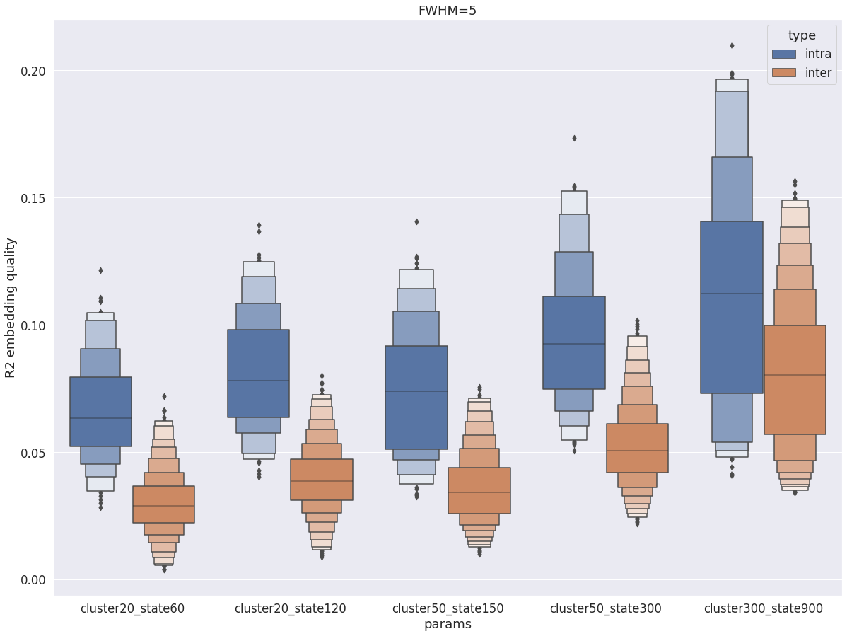
intra vs inter subject R2
Finally, intra-subject R2 is still higher than inter-subject R2, but compared with the cortex, there is a lot of overlap between the two distributions for all parameters cluster and state, with maximal overalp being observed again with cluster-300_state-900.
val_r2 = pd.read_pickle(dypac60)
val_r2 = val_r2.append(pd.read_pickle(dypac120))
val_r2 = val_r2.append(pd.read_pickle(dypac150))
val_r2 = val_r2.append(pd.read_pickle(dypac300))
val_r2 = val_r2.append(pd.read_pickle(dypac900))
val_r2 = val_r2.append(pd.read_pickle(inter60))
val_r2 = val_r2.append(pd.read_pickle(inter120))
val_r2 = val_r2.append(pd.read_pickle(inter150))
val_r2 = val_r2.append(pd.read_pickle(inter300))
val_r2 = val_r2.append(pd.read_pickle(inter900))

fig = plt.figure(figsize=(20, 15))
sns.boxenplot(data=val_r2, x='params', y='r2', hue='type', scale='area')
plt.ylabel('R2 embedding quality')
plt.title(f'FWHM={fwhm}')
Text(0.5, 1.0, 'FWHM=5')
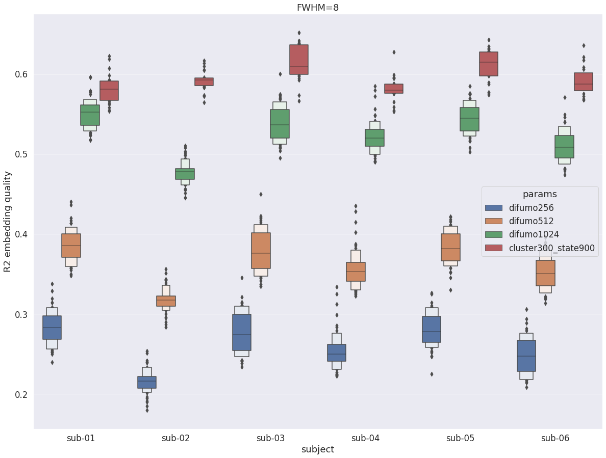
R2 with fwhm=8
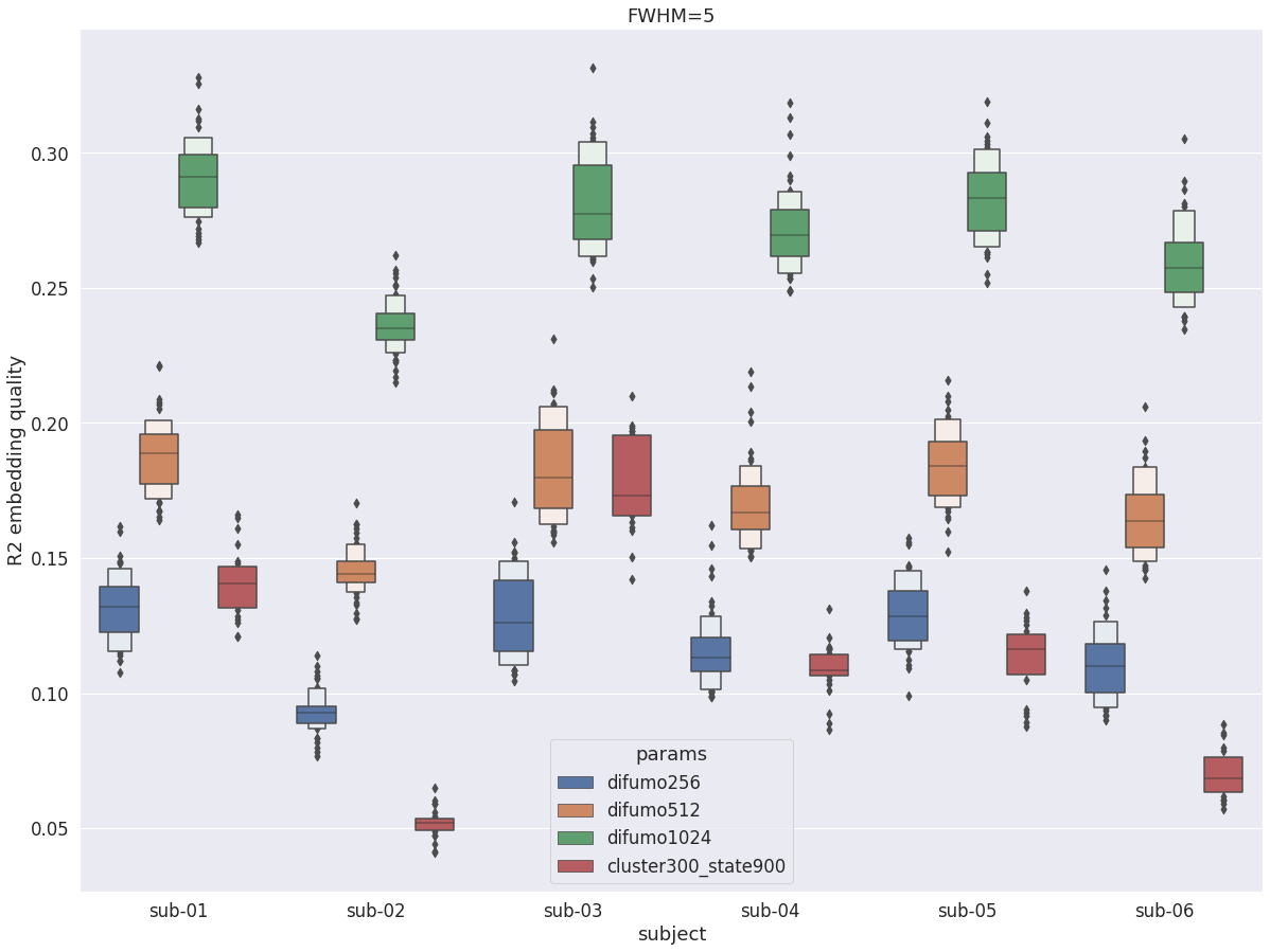
DYPAC intra vs DIFUMO
Interstingly, with fwhm=8, the results change almost completely. DYPAC parcellation (cluster-300_state-900) now outperforms even difumo1024 for every subjects, in a way that is similar to what was observed in the cortex.
path_results = '/data/cisl/pbellec/cneuromod_embeddings/xp_202012/r2_friends-s01_central/'
fwhm = 8

# DYPAC
dypac60  = os.path.join(path_results, f'r2_fwhm-intra_fwhm-{fwhm}_cluster-20_state-60.p')
dypac120 = os.path.join(path_results, f'r2_fwhm-intra_fwhm-{fwhm}_cluster-20_state-120.p')
dypac150 = os.path.join(path_results, f'r2_fwhm-intra_fwhm-{fwhm}_cluster-50_state-150.p')
dypac300 = os.path.join(path_results, f'r2_fwhm-intra_fwhm-{fwhm}_cluster-50_state-300.p')
dypac900 = os.path.join(path_results, f'r2_fwhm-intra_fwhm-{fwhm}_cluster-300_state-900.p')

# DYPAC inter-subject
inter60  = os.path.join(path_results, f'r2_fwhm-inter_fwhm-{fwhm}_cluster-20_state-60.p')
inter120 = os.path.join(path_results, f'r2_fwhm-inter_fwhm-{fwhm}_cluster-20_state-120.p')
inter150 = os.path.join(path_results, f'r2_fwhm-inter_fwhm-{fwhm}_cluster-50_state-150.p')
inter300 = os.path.join(path_results, f'r2_fwhm-inter_fwhm-{fwhm}_cluster-50_state-300.p')
inter900 = os.path.join(path_results, f'r2_fwhm-inter_fwhm-{fwhm}_cluster-300_state-900.p')

# DIFUMO
difumo256  = os.path.join(path_results, f'r2_fwhm-difumo256_fwhm-{fwhm}.p')
difumo512  = os.path.join(path_results, f'r2_fwhm-difumo512_fwhm-{fwhm}.p')
difumo1024 = os.path.join(path_results, f'r2_fwhm-difumo1024_fwhm-{fwhm}.p')

# MIST
mist197 = os.path.join(path_results, f'r2_fwhm-mist197_fwhm-{fwhm}.p')
mist444 = os.path.join(path_results, f'r2_fwhm-mist444_fwhm-{fwhm}.p')

# Schaefer
schaefer = os.path.join(path_results, f'r2_fwhm-schaefer_fwhm-{fwhm}.p')

# Smith
smith70 = os.path.join(path_results, f'r2_fwhm-smith_fwhm-{fwhm}.p')
val_r2 = pd.read_pickle(difumo256)
val_r2 = val_r2.append(pd.read_pickle(difumo512))
val_r2 = val_r2.append(pd.read_pickle(difumo1024))
val_r2 = val_r2.append(pd.read_pickle(dypac900))

fig = plt.figure(figsize=(20, 15))
sns.boxenplot(data=val_r2, x='subject', y='r2', hue='params', scale='area')
plt.ylabel('R2 embedding quality')
plt.title(f'FWHM={fwhm}')
Text(0.5, 1.0, 'FWHM=8')
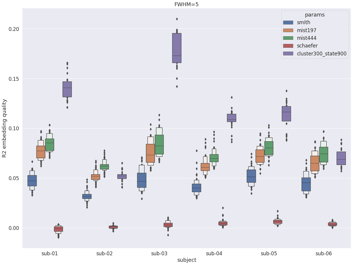
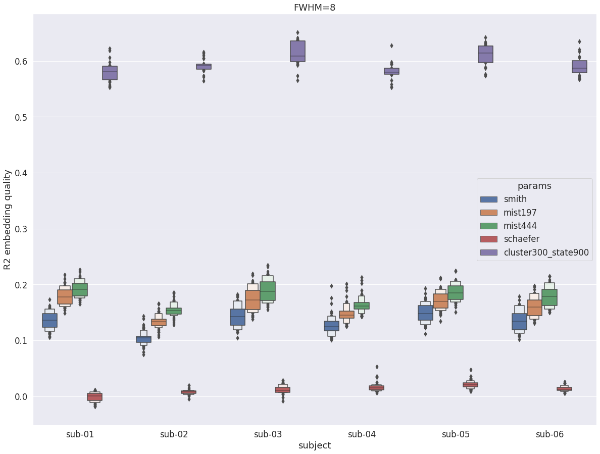
DYPAC intra vs other group parcellations
When compared with traditional group parcellations, with fwhm=8, DYPAC parcellation (cluster-300_state-900) now lead to a massive increase of about 200% in R2.
val_r2 = pd.read_pickle(smith70)
val_r2 = val_r2.append(pd.read_pickle(mist197))
val_r2 = val_r2.append(pd.read_pickle(mist444))
val_r2 = val_r2.append(pd.read_pickle(schaefer))
val_r2 = val_r2.append(pd.read_pickle(dypac900))

fig = plt.figure(figsize=(20, 15))
sns.boxenplot(data=val_r2, x='subject', y='r2', hue='params', scale='area')
plt.ylabel('R2 embedding quality')
plt.title(f'FWHM={fwhm}')
Text(0.5, 1.0, 'FWHM=8')
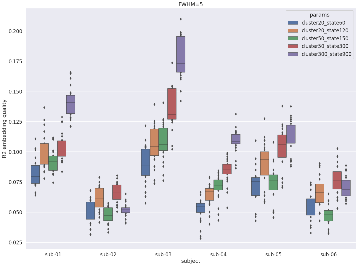
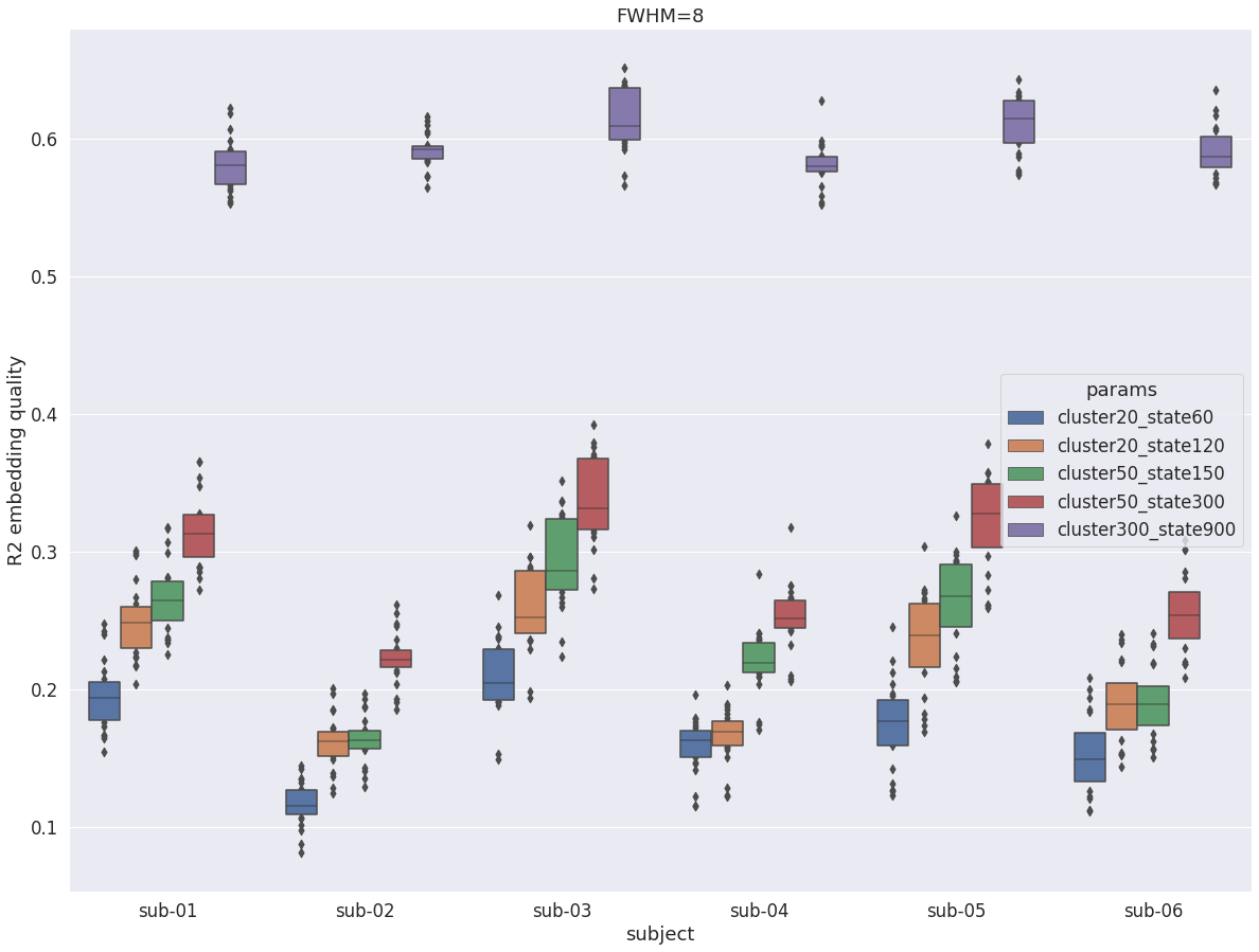
DYPAC multi-resolution
When looking at the impact of parameters cluster and state, the usual increase in R2 for larger state is observed. However, there is now a very large boost in R2 for all subjects when going from cluster-50_state-300 to cluster-300_state-900, which is very different from what observed in the cortex, or in the central structures with fwhm=5.
val_r2 = pd.read_pickle(dypac60)
val_r2 = val_r2.append(pd.read_pickle(dypac120))
val_r2 = val_r2.append(pd.read_pickle(dypac150))
val_r2 = val_r2.append(pd.read_pickle(dypac300))
val_r2 = val_r2.append(pd.read_pickle(dypac900))

fig = plt.figure(figsize=(20, 15))
sns.boxenplot(data=val_r2, x='subject', y='r2', hue='params', scale='area')
plt.ylabel('R2 embedding quality')
plt.title(f'FWHM={fwhm}')
Text(0.5, 1.0, 'FWHM=8')
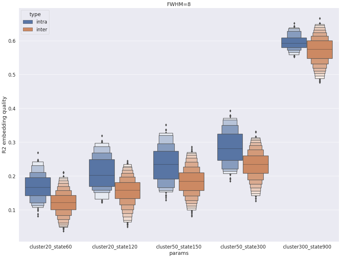
Intra vs inter subject R2
Finally, the intra-subject R2 values remain larger than inter-subject R2, but there is now a lot of overlap between the two distributions, and for cluster-300_state-900 the difference has become small. This is a trend observed in the cortex and with fwhm=5 as well, but it is much stronger with fwhm=8 in the central structure, suggesting that a single group parcellation may be appropriate in central structures at such low resolution.
val_r2 = pd.read_pickle(dypac60)
val_r2 = val_r2.append(pd.read_pickle(dypac120))
val_r2 = val_r2.append(pd.read_pickle(dypac150))
val_r2 = val_r2.append(pd.read_pickle(dypac300))
val_r2 = val_r2.append(pd.read_pickle(dypac900))
val_r2 = val_r2.append(pd.read_pickle(inter60))
val_r2 = val_r2.append(pd.read_pickle(inter120))
val_r2 = val_r2.append(pd.read_pickle(inter150))
val_r2 = val_r2.append(pd.read_pickle(inter300))
val_r2 = val_r2.append(pd.read_pickle(inter900))

fig = plt.figure(figsize=(20, 15))
sns.boxenplot(data=val_r2, x='params', y='r2', hue='type', scale='area')
plt.ylabel('R2 embedding quality')
plt.title(f'FWHM={fwhm}')
Text(0.5, 1.0, 'FWHM=8')